Research Article, J Biodivers Manage Forestry Vol: 9 Issue: 1
The Effects of Cell Size and Filtering Range on Automatically Extracted Tree Number and Average Tree Height Using Light Detection and Ranging Data in Fusion/LDV
Hiromi Shiota1*, Kazuhiro Tanaka2 and Keiko Nagashima1
1Graduate School of Life and Environmental Sciences, Kyoto Prefectural University, 1-5 Hangi-cho Shimogamo, Sakyo-ku, Kyoto, Japan
2Department of Bioenvironmental Science, Kyoto University of Advanced Science, 1-1 Nanjo Otani, Sogabe-cho, Kameoka, Japan
*Corresponding Author : Hiromi Shiota, Graduate School of Life and Environmental
Sciences
Kyoto Prefectural University, 1-5 Hangi-cho Shimogamo, Sakyo-ku, Kyoto
606-8522, Japan
Tel/Fax: +81-77-525-2075; E-mail: hshiota@msn.com
Received: December 26, 2019 Accepted: January 10, 2020 Published: January 17, 2020
Citation: Shiota H, Tanaka K, Nagashima K (2020) The Effects of Cell Size and Filtering Range on Automatically Extracted Tree Number and Average Tree
Height Using Light Detection and Ranging Data in Fusion/LDV. J Biodivers Manage Forestry 9:1. doi: 10.37532/jbmf.2020.9(1).226
Abstract
Objective: The use of airborne light detection and ranging (LiDAR) data is common in forest structure analyses. This study investigated the differences in tree number extraction and tree height measurements obtained using LiDAR data, employing different parameters (cell size, filter type, and filter range) and local maxima (LM) method. Tree numbers were extracted and parameter combinations resulting in values closest to the observed data were identified.
Method: For the two study sites, a Japanese cedar forest and a Japanese cypress forest, digital elevation model has a resolution of 1 m, and Digital Canopy Height Model (DCHM) calculated the difference using the resolution with varying parameters. Different combinations of cell size, filter type, and filter range parameters were employed for tree number extraction using DCHM. A total of 108 combinations were investigated, including 9 cell sizes (0.1 m to 0.5 m, at 0.05 m intervals) for the digital surface model, 2 filter types (median and average) for the LM method, and 6 LM ranges (from 3×3 to 13×13). Average tree height was calculated concurrently with tree number extraction, and results were compared with those of the on-site survey.
Results: An exponential trend was observed for the extracted tree numbers, with the number of extracted trees increasing for smaller cell sizes and decreasing for larger cell sizes. No significant differences were observed between the filter types. Tree height tended to measured values was close to the actual values observed on-site.
Conclusion: Extracted tree numbers close to the actual values were obtained near the shortest distance point from the origin (i.e., near the concave point) on the exponential (inverse) graph, suggesting that tree numbers can be estimated using LiDAR data.
Keywords: LiDAR; DCHM; LMF; Forest Inventory; Forest Planning; Tree Height Measurement; Fusion/LDV
Introduction
Airborne light detection and ranging (LiDAR) is a technology developed for measuring height of objects on the ground surface by irradiating numerous lasers from the air towards the ground and determining the laser reflection time (i.e., the return pulse). These measurements provide three-dimensional positional information across broad spatial ranges. In forests, LiDAR data can be used to measure the tree height, extract the number of trees (i.e., stand density), and estimate timber volume. For effective and efficient management of forest resources, many studies have examined the practical use of data obtained using airborne LiDAR [1,2]. In addition to Japan, several studies and projects have been undertaken in the United States, Canada, and northern Europe, since the 1990s [3-5].
There are two main methods for analyzing LiDAR data, namely, area-based approach (ABA) and individual tree detection (ITD) method. ABA is used to estimate area-based information, such as average tree number and tree height.
ABA is already being applied in several locations [3,6], and previous studies, conducted in different countries, have reported its accuracy [6,7]. Conversely, ITD is used to extract information relating to individual trees. ITD has been receiving increasing attention, as it can provide more concrete information than ABA [8]. For extracting information based on ITD, the usual process is to first develop the digital canopy height model (DCHM), and then apply methods such as the local maxima (LM) method, the watershed method, the valleyfollowing method, or the hybrid method, to combine the DCHM data with high-precision aerial photography.
Several studies have demonstrated the effectiveness of this method in extracting tree numbers and measuring tree heights [2,5,9]. However, few studies have discussed the effects of the differences in applied parameters (e.g., cell size, filter type, range of the method, etc) on the results [10]. For instance, previous studies applying LM used a cell size of 0.25 m to develop the DCHM [5,10,11], however, few studies have examined the appropriate cell size for developing the DCHM for extracting tree numbers.
Here, we used the LM method with a sampling density of 4 points/ m2 of LiDAR data, for two forest stands differing in age and species, i.e., a 0.37 ha forest of 42-year-old Japanese cedar (Cryptomeria japonica) in a national forest at Mt. Ansyoji, Kyoto, and a 0.75 ha forest of 97-yearold Japanese cypress (Chamaecyparis obtusa) in a national forest at Mt. Koyama, Kyoto, in order to assess the appropriate parameters. We then compared the results of the extracted tree numbers and automatically calculated tree heights with those obtained from the on-site survey to determine the most appropriate parameter combinations that resulted in measurements close to the actual values. We further compared the appropriate parameter combinations of the two stands, and discussed the effects of tree species on these parameter combinations.
Materials and Methods
Study area
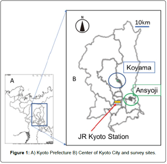
Mt. Ansyoji: The national forest at Mt. Ansyoji (19-21compartments, 16 ha) is located to the north of Yamashina Ward in Kyoto (Figure 1).
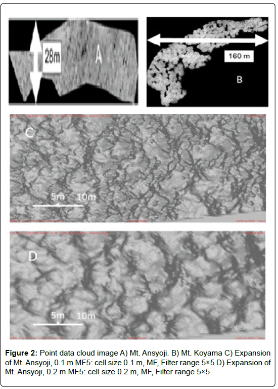
Topographically, elevation of the forest is higher on the north, south, and west sides, i.e., the area gradually slopes to the east. The surveyed plot [0.3 ha] (Figure 2A) is a catchment for water flowing from the north, south, and west sides towards the east. The forest is a 42-years-old woodlot for Japanese cedar, and had been thinned twice before the LiDAR data was acquired. A plot was installed by surveying the site, using the boundary markers of the national forest.
Mt. Koyama: The national forest at Mt. Koyama, a mountain known as the “holy object of worship” of the Kamigamo Shrine, is located on its southwest slope. The land southeast to the surveyed site was bare, without any forest (Figure 2B). Topographically, the elevation of the national forest is higher on the north side and lower on the south side. This forest is a 97 years old woodlot for Japanese cypress, and had been thinned twice before the LiDAR data was acquired. The survey plot [0.75 ha] (Figure 2B) was installed by surveying the site using coordinates whose fiducial points were artificial structures in proximity of the plot (Figures 2A and 2B).
Fusion/LDV: Fusion/LDV (V3.8) is a freely available software program for analyzing LiDAR data from forest resources, developed by Robert J. McGaughey of the USDA Forest Service Pacific Northwest Research Station. This program uses an algorithm based on the LMF (Local Maximum Filtering) method to automatically extract tree number, measure tree height, and record tree coordinates.
LiDAR data: LiDAR data and aerial photographs were acquired on November 24 and 26, 2013, using a helicopter-borne laser scanner (HARRIER56, Trimble) operated by Asia Air Survey, Japan. LiDAR data were acquired with the following specifications: average flight speed 20 m/s, flight altitude 550-1360 m above sea level, pulse frequency 120 kHz, scan frequency 44.74 kHz, scan angle ± 30°, with over 50% overlap between the courses. The LiDAR system registered two echoes of the laser beam, i.e., the first and last pulses. The laser sampling density of the LiDAR data was configured for acquiring greater than 4 points/m2. A Global Navigation Satellite System base control station was located at Kyoto Sakyo 2, code EL05235466102.
Methodology
Field survey: We established one survey plot at each study site. The boundary coordinates of each plot were obtained using GPS and Google Earth. We evaluated the tree number, tree height, and crown width for all trees in the plot, and then obtained the average tree height and average crown width for each plot. Information regarding the tree species and forest age was obtained from the forest register. The tree height was measured using Vertex II and III, and the crown width was obtained by measuring the distance between the stem and the tip of the raw branch in all four directions (east, west, south, and north of the stem), and then averaging the four distances.
LiDAR data analyses: Plot polygons were created using plot boundary coordinates, and plot area was calculated using geographic information system (GIS).
The density of standing trees was obtained from the plot area and tree number. In addition, the relative spacing index (Sr), indicating the degree of forest congestion, was calculated from the average tree height and number of standing trees per ha (N), using the following formula:

LAS (LASer) data corresponding to the plot was obtained by clipping the original LAS data from LiDAR, using the plot polygons. The digital terrain model (DTM) was developed by extracting the last pulse from the clipped LAS data.
The DCHM was developed from the LAS and DTM data, using the “Canopy Model” command in Fusion/LDV. Once the DCHM was obtained, we changed the parameters of cell size, filter type, and filter range, as follows: nine cell sizes (every 0.05 m, from 0.1 m to 0.5 m), two filter types (average value filter [AF] and median value filter [MF]), and 6 filter ranges (3 × 3, 5 × 5, 7 × 7, 9 × 9, 11 × 11, and 13 × 13 cells), totaling 108 combinations. DCHM images are presented in Figures 2C and 2D.
The 108 DCHM were assessed by the LMF method, applied using the “CanopyMaxima” command in Fusion/LDV. Trees were automatically extracted, and tree number and the median and average values for tree height were calculated. For consistency, the combinations are expressed in the order of cell size, filter type, and filter range, e.g., in 0.2 m MF5, 0.2 m indicates cell size, MF indicates filter type MF, and 5 indicate filter range of 5×5 (Table 1).
| Field | Mt. Ansyoji | Mt. Koyama | |
|---|---|---|---|
| Number of return points | Unclassified | 91,362 | 2,86,492 |
| Ground | 4,379 | 25,337 | |
| Total | 95,741 | 3,11,897 | |
| First return | 73,270 | 2,12,800 | |
| Coordinate | Minimum X | -17576.02 | -22609.59 |
| Minimum Y | -110406.77 | -102382.98 | |
| Maximum X | -17404.68 | -22,448.90 | |
| Maximum Y | -110378.96 | -102275.09 | |
| Elevation (m) | Minimum | 139.22 | 166.97 |
| Maximum | 177.94 | 206.69 |
Table 1: LiDAR data catalog by field. Data: JGD2011_Japan_Zone_6.
Influence of parameter combinations on the estimation results:
Tree numbers: The trends in the extracted tree numbers due to differences in cell size, filter type, and filter range were interpreted by creating a contour graph based on the automatically extracted tree number data. A line graph of the number of extracted trees was created for each combination of filter type (AF, MF) and filter ranges. For this, the cell size was plotted on the X axis and the number of extractions was plotted on the Y axis. As the shape of the graph was considered to approximate to an inversely proportional graph, a power approximate curve was created for each filter type and filter range, using Excel, for estimating the actual tree number (Figure 3).
Tree height: In order to investigate the accuracy of the automatically calculated tree heights, the distribution of tree numbers by height class, based on the best parameter combination obtained from tree number extraction, was compared to that obtained from the field data. Using the average (AV) and median (MV) values of the automatically measured tree height, the differences in tree height due to cell size, filter type, and filter range were interpreted by creating a contour graph. A box chart was created for comparing the results of AV and MV by filter type and filter range.
Results and Discussion
Extracted tree number
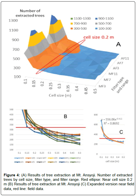
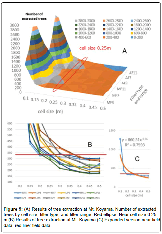
•From the extraction of tree number by cell size, filter type, and filter range, it became evident that as the cell size decreased, the number of extracted trees increased (Table 2). This tendency was confirmed by contour graphs of both Mt. Ansyoji (Figure 4A) and Mt. Koyama (Figure 5A). For small cell sizes and filter ranges of 7 × 7 and 9 × 9, the extracted value was nearly 1.5 to 2 times greater than those extracted using other ranges. This tendency was further confirmed in AF and MF, for both the sites.
| Cell size | MF3 | MF5 | MF7 | MF9 | MF11 | MF13 | AF3 | AF5 | AF7 | AF9 | AF11 | AF13 |
|---|---|---|---|---|---|---|---|---|---|---|---|---|
| 0.1 | 614 | 676 | 999 | 976 | 853 | 850 | 590 | 716 | 1110 | 1031 | 903 | 871 |
| 0.15 | 329 | 370 | 428 | 435 | 400 | 395 | 331 | 403 | 469 | 459 | 433 | 399 |
| 0.2 | 279 | 313 | 337 | 349 | 341 | 354 | 279 | 306 | 359 | 366 | 341 | 345 |
| 0.25 | 254 | 283 | 308 | 301 | 288 | 270 | 265 | 312 | 326 | 322 | 302 | 269 |
| 0.3 | 242 | 267 | 280 | 254 | 243 | 242 | 258 | 292 | 290 | 256 | 243 | 223 |
| 0.35 | 242 | 265 | 276 | 249 | 242 | 239 | 244 | 274 | 246 | 225 | 203 | 187 |
| 0.4 | 232 | 260 | 240 | 220 | 215 | 218 | 246 | 260 | 239 | 206 | 187 | 179 |
| 0.45 | 234 | 252 | 224 | 187 | 192 | 234 | 238 | 249 | 213 | 188 | 170 | 170 |
| 0.5 | 241 | 255 | 211 | 202 | 197 | 205 | 241 | 247 | 198 | 165 | 166 | 152 |
Table 2A: Number of extracted trees. Red cell: Within ± 3% of field data. Field data: Mt. Ansyoji, 317.
| Cell size | MF3 | MF5 | MF7 | MF9 | MF11 | MF13 | AF3 | AF5 | AF7 | AF9 | AF11 | AF13 |
|---|---|---|---|---|---|---|---|---|---|---|---|---|
| 0.1 | 1260 | 1857 | 2779 | 2736 | 2137 | 1644 | 1277 | 2005 | 2938 | 2760 | 2125 | 1581 |
| 0.15 | 426 | 607 | 903 | 895 | 685 | 523 | 447 | 861 | 1167 | 991 | 710 | 536 |
| 0.2 | 324 | 395 | 488 | 458 | 379 | 363 | 339 | 541 | 633 | 499 | 396 | 340 |
| 0.25 | 327 | 405 | 428 | 366 | 322 | 304 | 333 | 470 | 454 | 377 | 334 | 289 |
| 0.3 | 315 | 388 | 348 | 302 | 269 | 251 | 337 | 397 | 344 | 292 | 257 | 217 |
| 0.35 | 313 | 348 | 316 | 265 | 232 | 245 | 327 | 354 | 302 | 251 | 209 | 201 |
| 0.4 | 296 | 318 | 273 | 225 | 229 | 222 | 308 | 311 | 271 | 215 | 187 | 184 |
| 0.45 | 286 | 293 | 243 | 224 | 206 | 248 | 301 | 288 | 229 | 189 | 177 | 171 |
| 0.5 | 293 | 293 | 226 | 223 | 255 | 241 | 303 | 279 | 213 | 192 | 177 | 173 |
Table 2B: Number of extracted trees. Red cell: Within ± 3% of field data; Mt. Koyama, 331.
Based on the linear graph (Figure 4B and Figure 5B) and the tree number extraction data, the optimal cell size, i.e., the cell size for which the extracted tree number was within ± 3% of the actual tree number, was 0.2-0.25 m at Mt. Ansyoji (317); (Figure 5 and Table 2), and 0.2-0.35 m at Mt. Koyama (331); (Figure 6 and Table 2).
The forest stand at Mt. Ansyoji is a cedar plantation, and cedar has a more obvious treetop than cypress, therefore, smaller cell sizes can be used for cedar forests. In addition, as evident from the tree density of both forests, Mt. Ansyoji was more crowded (1,056 trees/ha, Sr:13) than Mt. Koyama (441 trees/ha, Sr:22.1); and the average crown width at Mt. Ansyoji (4 m); was about 1 m less than that at Mt. Koyama (4.95 m); (Table 3).
| Field | Mt. Ansyoji | Mt. Koyama | ||
|---|---|---|---|---|
| Field data | Elevation (m) | 146–150 | 170-180 | |
| Area (ha) | 0.3 | 0.75 | ||
| Species | Japanese cedar | Japanese Cypress | ||
| Tree age | 42 | 97 | ||
| No. of tree | 317 | 331 | ||
| Stand Density | 1,056 | 441 | ||
| number/ha | ||||
| Average | 4 | 4.95 | ||
| crown width (m) | ||||
| Sr | 13 | 22.1 | ||
| Tree height (m) | Average | 23.6 | 21.6 | |
| Median | 23.6 | 22.6 | ||
| LMF | Tree height (m) | 23.7 | 21.1 | |
| Cell size (m) | 0.2 | 0.25 | ||
| Filter type | MF | AF | ||
| Filter range | 5 × 5 | 3 × 3 | ||
| Number of extracted trees by upper parameter | 313 | 333 | ||
| Survey month | Oct, Nov, 2014 | Mar, Apr, 2015 |
Table 3: Field data and automatically extracted data.
As crowding increases in a stand, the crown size of individual trees decreases. The cell size, which is a unit for detecting the maximum height point to extract tree numbers by LMF, strongly relates to the crown size. This is because treetops of small crowns cannot be detected by large cell sizes, as only the treetop of the largest tree, among the several trees included in the huge cell, will be detected. Therefore, a smaller appropriate cell size at Mt. Ansyoji than that at Mt Koyama would be suitable.
The linear graph further indicated that the optimal cell size for each combination of filter type and filter range was around the concave conversion point (Figure 4B and Figure 5B). For example, extracted tree numbers closest to the actual tree numbers were obtained with the parameter combination of 0.2 m MF5 at Mt. Ansyoji (313 extracted trees), and 0.25 m AF5 at Mt. Koyama (333 extracted trees).
The calculated power approximated curve was strongly correlated to the linear graph (correlation coefficient: 0.8692 at Mt. Ansyoji, 0.7593 at Mt Koyama). This might indicate the suitability of the power approximated curve in determining the appropriate cell size for estimating the number of trees, if the curve could be applied to other stands with the same tree species and tree density. Further research is required to confirm if the curve would be the same for such stands, and to calculate the curve for different stands and different tree densities.
Average tree height
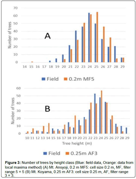
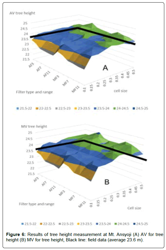
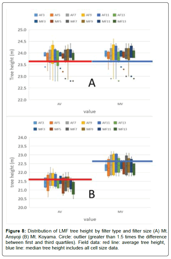
The actual average tree height at Mt. Ansyoji was 23.6 m, while that obtained by the LMF method was 23.7 m (parameter combination 0.2 m MF5); (Table 3), which was 0.1 m greater than the actual height. The tree height distribution of this parameter combination was very similar to that observed during the field survey (Figure 3A); however, it shifted towards a relatively higher height, greater by 1 m. According to the contour graph, the measured tree height was lower than the actual tree height when the cell size was small, and it exhibited a tendency to increase with increasing cell size, for both AV and MV (Figure 6). Outliers (more than 1.5 times the difference between the first and third quartiles) were detected in the box graph, in the lower tree height for both AV and MV. The difference in tree height between AF and MF was less than 0.1 m. The average tree height obtained by LMF was about 0.2-0.5 m higher than the actual tree height. In addition, when the filter range was narrow, the difference in the measured average tree height was small (Figure 6).
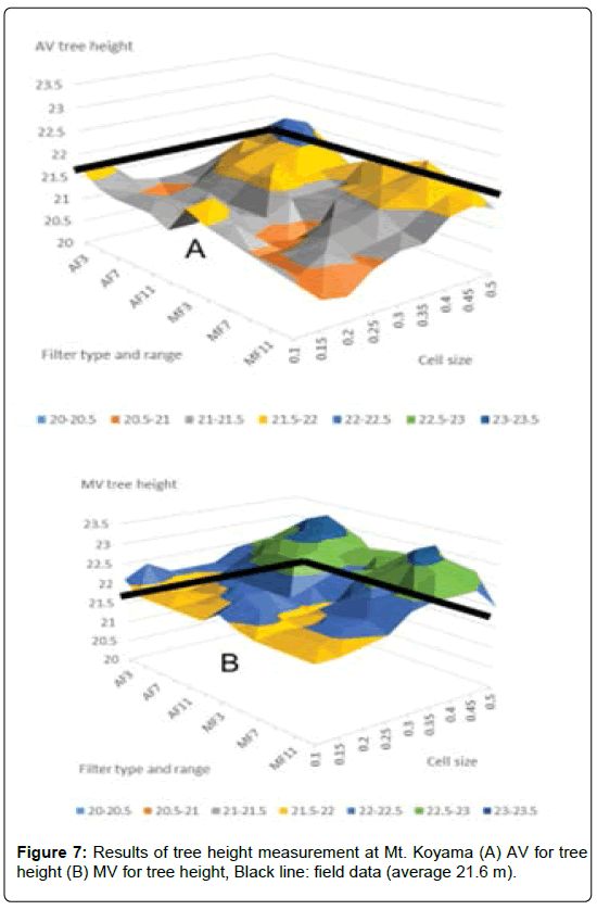
The average tree height obtained by the LMF method at Mt. Koyama (parameter combinations shown in Table 3[cell size: 0.25, AF3)] was 21.1 m, which was 0.5 m less than the actual height of 21.6 m. The distribution of tree height for this parameter combination was different from the actual tree height distribution. Over- and underestimation were observed for low tree heights. The contour graph revealed that the measurements tended to be slightly higher for small cell size and filter range.
For cell sizes ranging from 0.2 to 0.3 m, both AV and MV were underestimated (Figure 7). No outliers were observed in the box graphs of AV and MV. Measured MV were about 0.8 m higher than the actual values in all filter types and filter ranges (Figure 8), while measured AV were found to be similar to the actual values (Figure 7 and 8).
The exact reason for the different tendencies observed at Mt. Ansyoji and Mt. Koyama is not known. However, tree species could be one of the factors, as Mt. Ansyoji is a Japanese cedar stand and Mt. Koyama is a Japanese cypress stand. As cypress has a gentler crown than cedar, the height differences might be smaller even if the extracted treetops were different from the actual ones. This might be the reason for no outliers being detected in the cypress box charts.
The age of the forest and tree density could be other factors influencing the tendency observed for tree height measurements. Further studies comparing the age and density of stands of the same species are required to conclusively determine the reason behind the different tree height measurement tendencies observed in this study.
Overall, the measured average tree height was within ± 1 m of the actual tree height for all parameter combinations used, suggesting that it can be used for forest resource analysis. Furthermore, our results indicated that AV and MV could be used for measuring cedar tree height; however, AV might be more suitable for cypress stands.
Conclusion
This study investigated different parameter combinations for extracting tree numbers and automatically calculating tree heights, for developing DCHM. Smaller cell sizes resulted in greater number of trees being extracted, and cell size was the most important factor influencing the extracted tree numbers. The most appropriate cell size for Mt. Ansyoji was smaller than that for Mt. Koyama, which might be attributed to the differences in tree density and crown size of these forests. The power approximated curve, which was highly corelated with the linear graph, could be used to determine the appropriate cell size for estimating the tree number, if the curve could be applied to other stands with the same tree species and density.
The estimated tree heights were lower than the actual values for smaller cell sizes. However, the measured average tree height was within ± 1 m of the actual tree height, and we concluded that all parameter combinations might be suitable for estimating cedar tree height; however, AV is recommended for use in cypress stands. Further research is required to verify if the same tendencies occur in other stands with the same tree species and tree density, and in different stands with different tree densities.
References
- Sasaki T (2012) Estimation of forest stand structures using airborne LiDAR. JALE 17: 43-55.
- Deng S, Katoh M (2016) Interpretation of forest resources at the individual tree level in Japanese conifer plantations using airborne LiDAR data. Remote Sens 8: 1-23.
- White JC, Wulder MA, Varhola A, Vastranta M, Coops NC, et al. (2013) A best practice guide for generating forest inventory attributes from airborne laser scanning data using an area-based approach. For Chron 89: 722-723.
- Laes D, Mellin T, Wilcox C, Anhold J, Maus P, et al. (2009) Mapping vegetation structure in the Pinaleño Mountains using LiDAR. RSAC-0118-RPT1.
- Lindberg E, Holmgren J, Olofsson K, Wallerman J, Olsson H (2010) Estimating tree lists from airborne laser scanning by combining single-tree and area-based methods. Int J Remote Sens 31: 1175-1192.
- Wulder MA, Coops NC, Hudak AT, Morsdorf F, Nelson R, et al. (2013) Status and prospects for LiDAR remote sensing of forest ecosystem. Can J Remote Sensing 39: 1-5.
- Næsset E (2015) Forestry Applications of Airborne Laser Scanning. In: Maltamo M, Vauhkonen J, Naesset E (eds.) Area-based inventory in Norway – from innovations to operational reality. Springer, Germany, pp: 215-240.
- Holopainen M, Vastaranta M, Hyyppä J (2014) Outlook for the next generation’s precision forestry in Finland. Forests 5: 1628-1694.
- Vauhkonen J, Ene L, Gupta S, Heinzel J, Holmgren J, et al. (2011) Comparative testing of single-tree detection algorithms under different types of forest. Forestry 85: 27-40.
- Endo T, Taguchi H, Baruah PJ, Sawada H (2009) Development of a methodology to extract individual trees in a Japanese Cider plantation using LiDAR data. SEISAN-KENKYU 61: 769-772.
- Hirata Y (2008) Research of forest structure with high-resolution remote sensing. Tokyo University.
